Project Report
Table of Contents
- Defining Correspondences
- Generating Morph Sequences
- Different Morphing Functions*
- Population Analysis
- Transforming Image Characteristics*
- Class Face Morph!*
- Making Caricatures
- Transformations & Transitions*
- Music Visualizer*#
# best part!
Introduction
In this project we'll explore image morphing! A morph is a simultaneous warp of the image shape and a cross-dissolve of the image colors where the warp is controlled by defining a correspondence between two pictures. We'll take a look at different morphing techniques, analyze population face shapes, generate fun caricatures and more.
Image Morphing Setup
1. Defining Correspondences
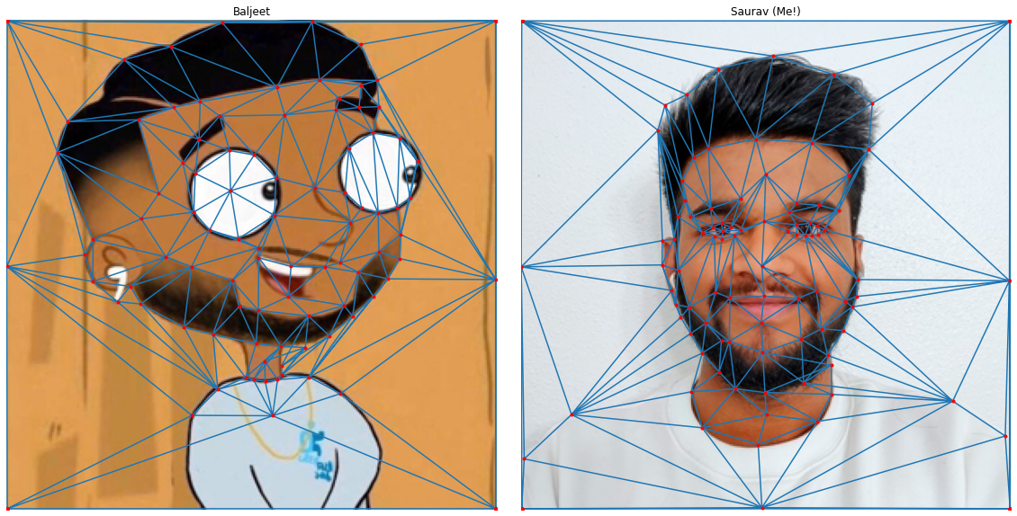
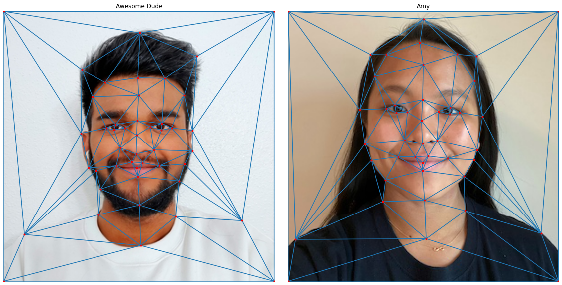
First, we will need to define pairs of corresponding points on the two images by hand (the more points, the better the morph, generally). In order for the morph to work we will need a consistent labeling of the two faces. We will label faces A and B in a consistent manner using the same ordering of keypoints in the two faces. Once we have the points on the two faces, we'll need to provide a triangulation of these points that will be used for morphing. I chose to use the Delaunay triangulation on the average point set of the two images since it does not produce overly skinny triangles.
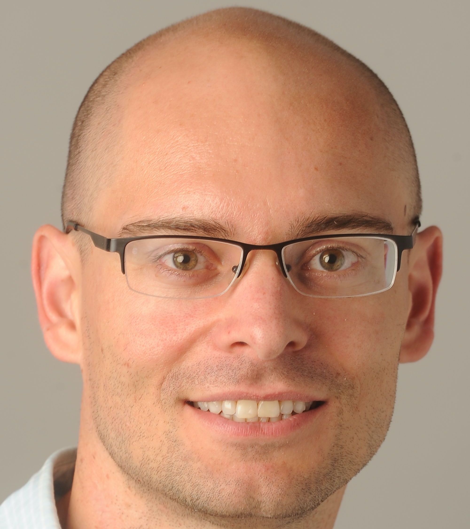
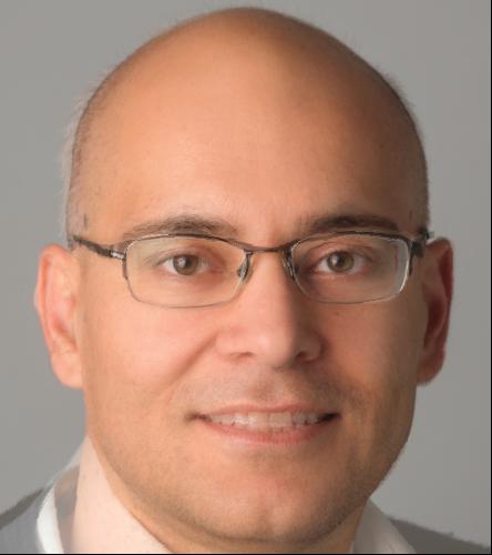
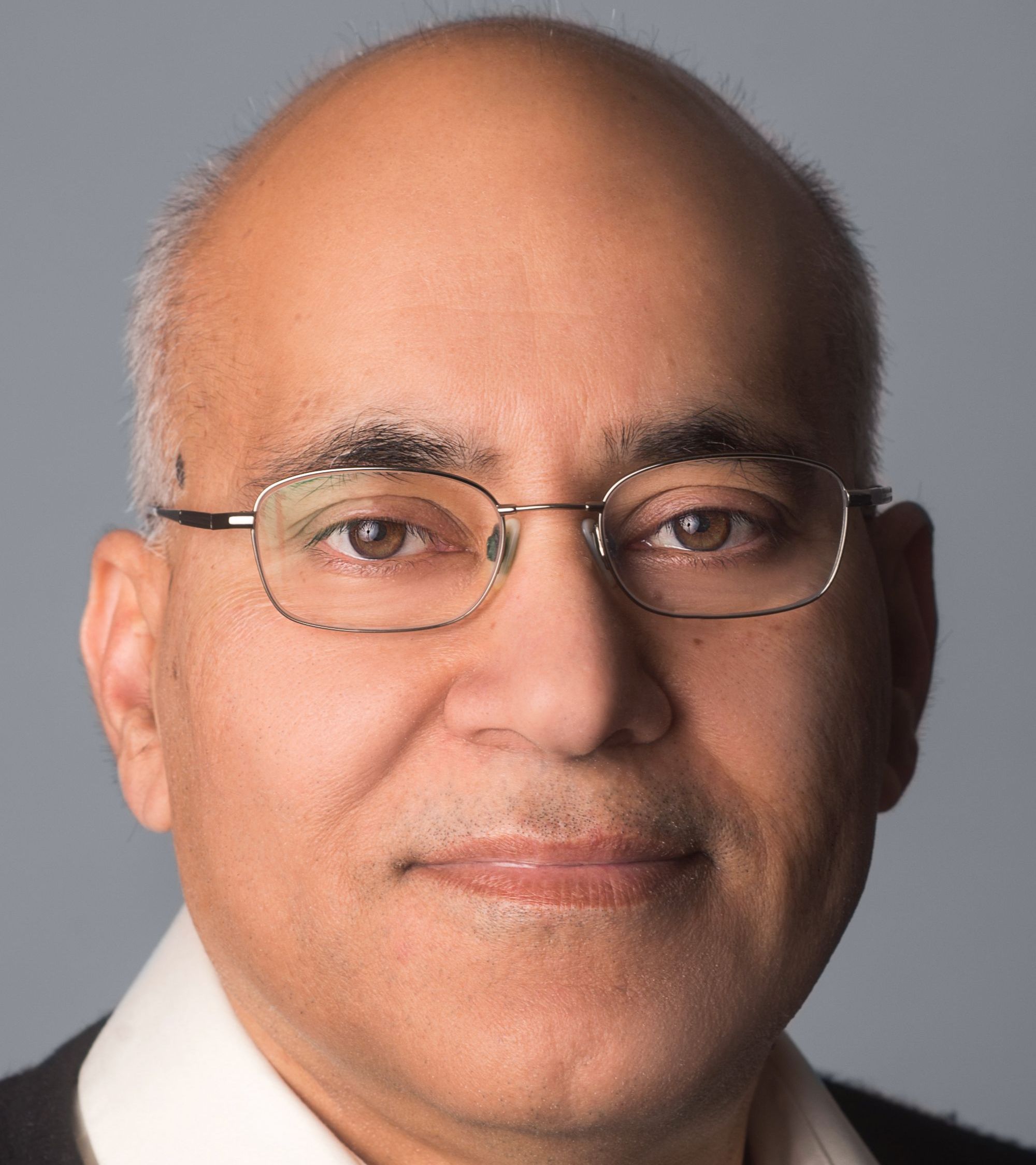
Note: For most of the project, we'll be working with the head shots of two awesome Berkeley EECS Professors, Professor Abbeel & Professor Malik. This is partly for consistency and mostly because manually defining correspondences is tedious and these were the pictures I went with when I started the assignment. You know people who would spend 242695 hours automating a 5 minute job instead of actually doing it? Yeah, I'm those people. I actually tried automating this process and failed so let's not even get into it. Wow we're just gonna enjoy the company of these professors and morph their faces even if it gets weird later (spoiler: it might 😉).
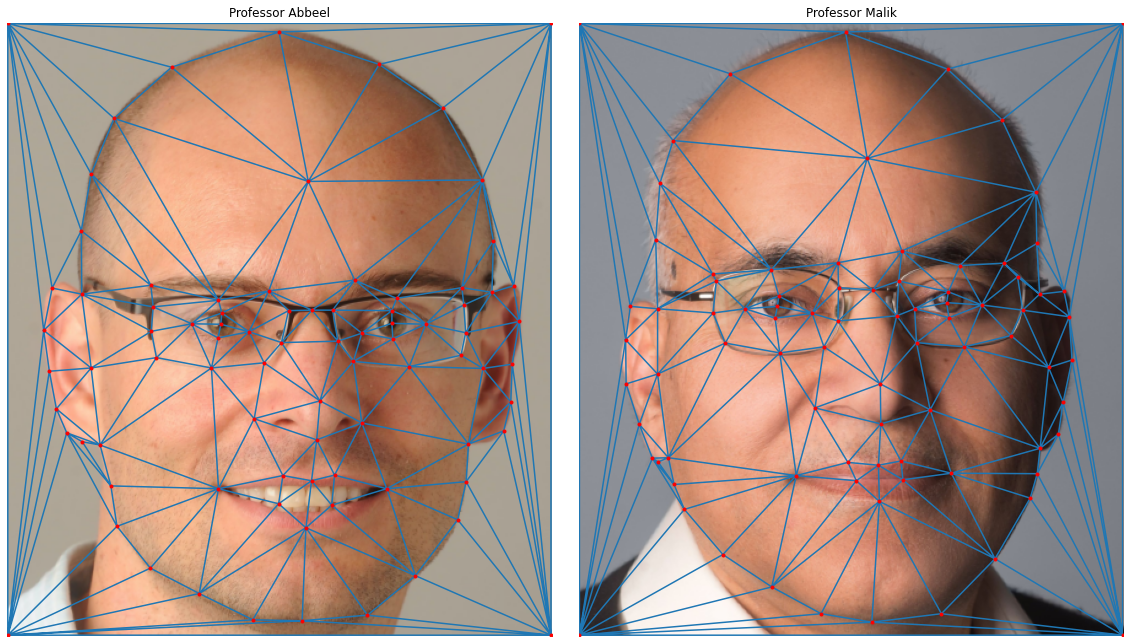
For these two images, I manually selected a shit ton of 84 points (including 4 corners) in both the images across different facial features and accessories (glasses) to set us up for a good morph. Once I got that, I used scipy library's Delaunay function to compute an abstract triangle representation on the mean point set of the two images which is shown above.
2. Generating Morph Sequences
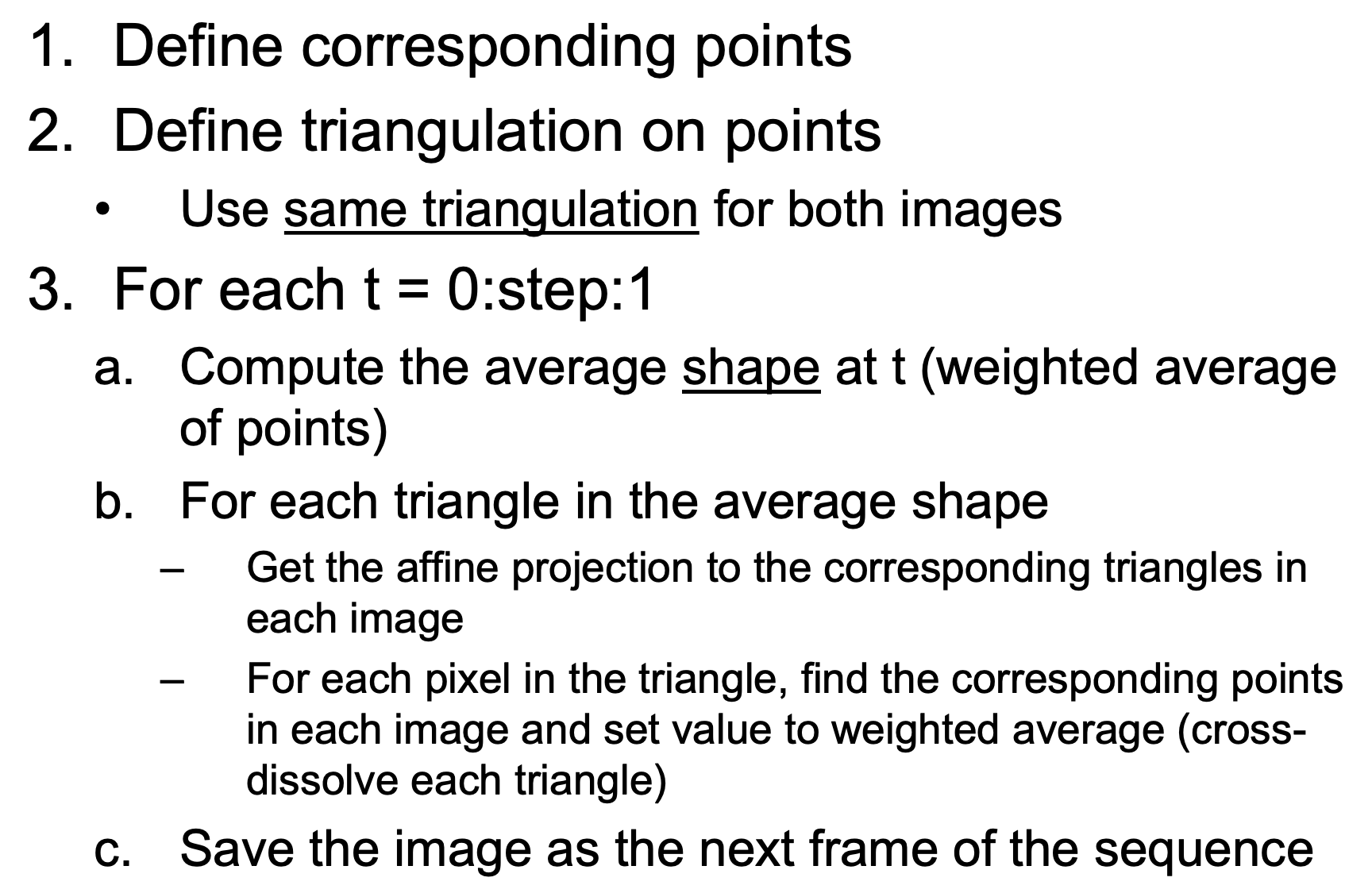
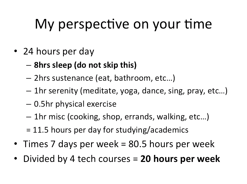
Before we compute the whole morph sequence, let's compute the mid-way face of these two images. This involves the following:
- Computing the average shape (a.k.a the average of each keypoint location in the two faces)
- Warping both faces into that shape
- Averaging the colors together.
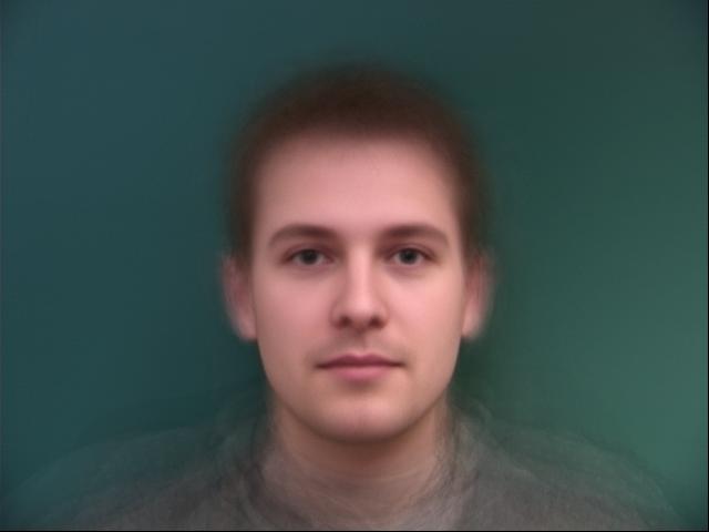
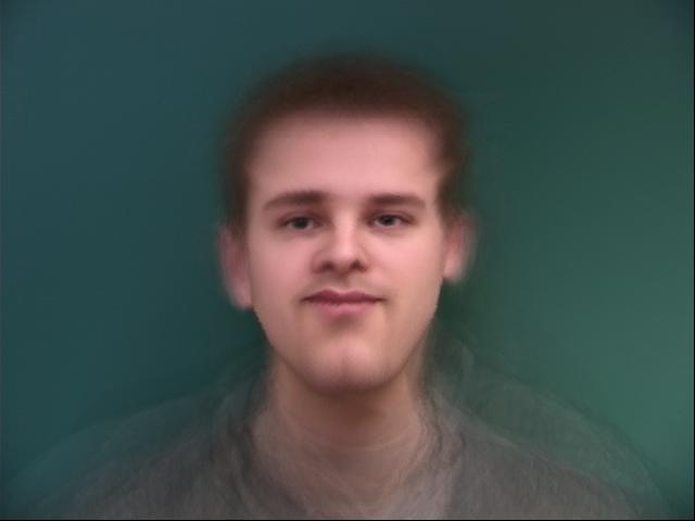
We found the mid-way face for our professors by warping both the faces to their average face shape and then blending both the faces together using equal weights.
Cool! It actually looks pretty realistic. Do note that the difference in quality is purely because I downsampled the images before processing to make the code run faster and to get lighter gif files for later.
<mini-rant> Why are gifs so big?? I know there are a lot of images but some quick math seems to show they are bigger than im_size*num_frames. All this overhead??? No wonder all gifs on the web look like trash smh </mini-rant>
Here is the result of using this algorithm to morph the images of Professor Abbeel & Professor Malik

3. Different Morphing Functions
We can play around with our base morph implementation a bit. There are two arguments we can tweak with our current algorithm, the warp factor & the morph factor. The warp factor tells the algorithm by how much to change the shape of our triangle in a given frame and the morph factor tells the algorithm how much we want to blend the two images for a frame. To understand this better, let's take a look at what changing one of these factors looks like while keeping the other constant at 1.


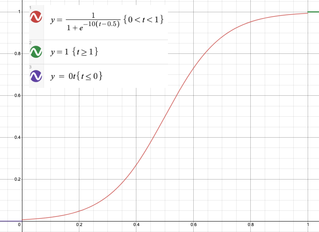
I had to play around with the domain and range of the function and clip it to make it work for our use case. The exact parametric sigmoid function and the plot of our new factor function is shown here.
| Linear Warp | Sigmoid Warp | |
| Linear Blend |
|
|
| Sigmoid Blend |

|

|
Comparing the different results, I don't think there's a clear winner here. It's really up to what you prefer. For this pair of images I think the Linear Blend + Linear Warp works quite well because the overall morph is fairly smooth so we get to see neat middle frames for longer. For other images where the transition isn't as smooth the linear map would likely be percieved worse than the sigmoid map because we would be spend a lot of time on frames which are not pleasing to look at. I annotated another set of pictures to showcase just this.


This morph isn't nearly as clean as the previous ones because the images are quite different from each other both in color and structure. The sigmoid morph looks better than the linear morph because it speeds through through the displeasing frames quicker.
I tried playing around with some other functions as well but they didn't really provide better results. A fun thing that I did try here was modeling the morph after a random walk.
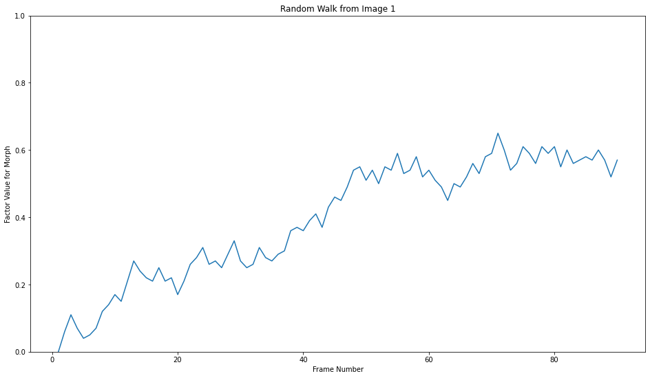
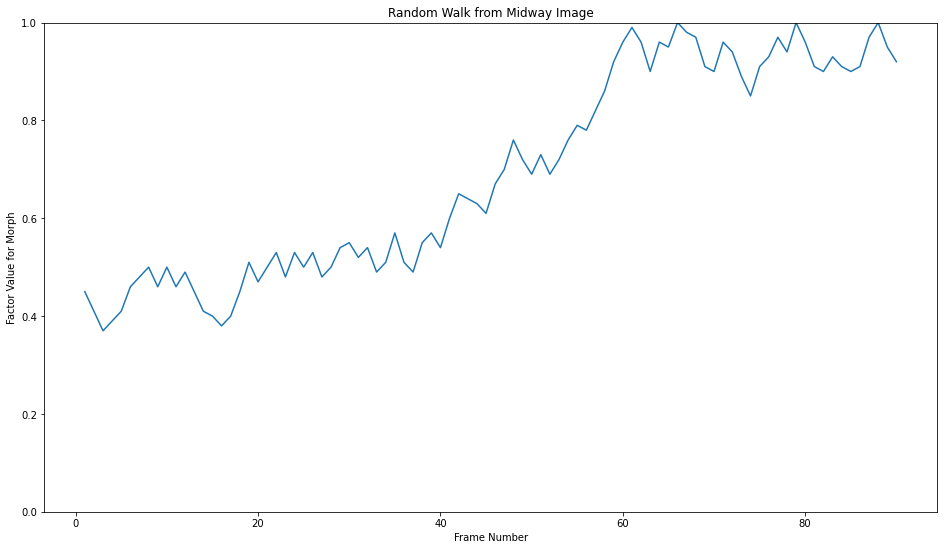
Why do this? No reason really, just seemed cool. Implementing the random morphs did give me a fun idea that I ended up working on a lot later so it was definitely worth :)
Fun with Face Morphing
1. Population Analysis
I analyzed a free data set of Danish faces meant for statistical models of shape available here for population facial feature analysis. We have 40 people in this dataset, we can start by finding the average face of this population. Computing the average face first finding the average face shape of the population, transforming all the faces into the average shape and then blending all the transformed faces together with equal weights.
2. Transforming Image Characteristics
Now I'll try to change some characteristics of my face using the features from the Danes dataset.


3. Class Face Morph!
We got 15 students from the class in our class morph video! My friend Rina morphed her face to mine and I morphed my face to Amy's.

List of students in order of appearance: Ritika Shrivastava, Megan Lee, Rina Lu, Saurav Mittal, Amy Hung, Cesar Plascencia Zuniga, Ron, Danji Liu, Saurav Shroff, Gurmehar Kaur, Avik Sethia, Devesh Agarwal, Yash Swarup Agarwal, Hannah Moore, and Matt Hallac.
Morphing Applications
1. Making Caricatures
Now we make caricatures of my face by extrapolating from the population mean that we calculated in the last section. We do this by finding the difference between the average face features & my face features and then adding it back to my face after scaling it.
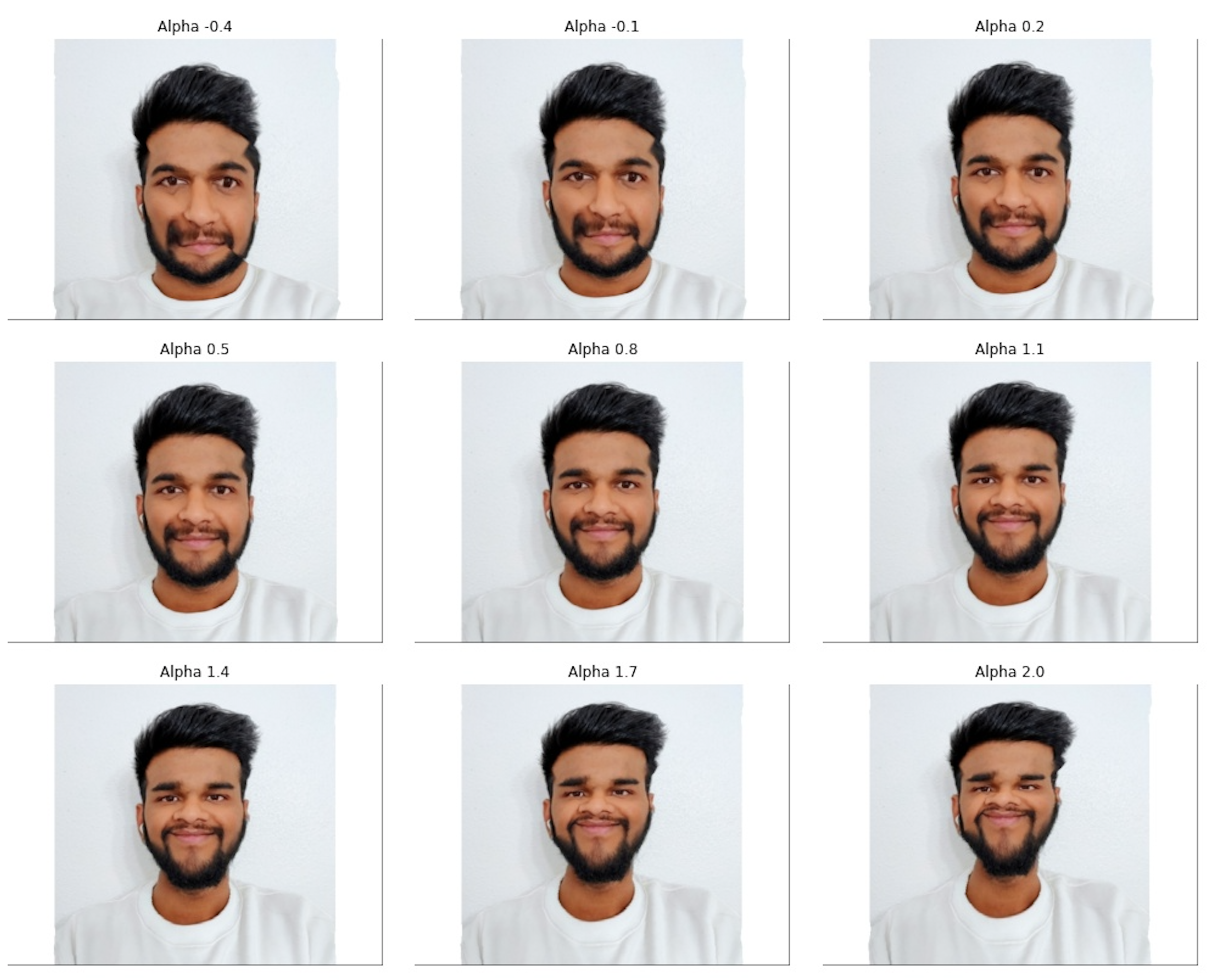
We see that the caricatures become more 'extreme' the further alpha deviates from 1 (which would yield the original image).
2. Transformations & Transitions
Transformations
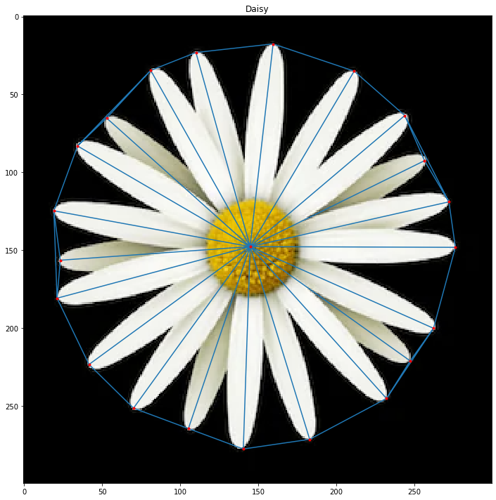
I wanted to see if it was possible to implement transformations using our morphing algorithm. For this, we have a new test subject – a pretty, symmetrical daisy :) As we aren't really morphing to any particular image for transformations, I used my warp-only morph which fixes the morph factor to 1. Here are some of the transformations I implemented.


All the transformations shown just use a single labeled pointset on the daisy (shown above). We generate our final point set (end state) through clever alterations of the original point set which lead to the desired effect. When the points move from their original location to their final location it appears as the image is being transformed.
Transitions
The goal here was to see if would be possible to implement Powerpoint-like slide transitions using our morphing algorithm. The process to generate transitions is pretty similar to what we did for transformations, but instead of doing a warp-only morph we now blend the images as well. I found best results with using a Linear Warp with Sigmoid Blend. This makes sense because the quick blend reduces the weird choppy middle frames (slides are likely different from each other) and the linear warp gives us a smooth structural transition from start to finish. Here are the test slides I used along with some transitions I tried out.


The first row of transitions just used the corners of the images for the transition sequences. 'Triangle Dust', on the other hand, has this very interesting effect as it used the Delaunay Triangulation on 256 randomly chosen points on both the images.
3. Music Visualizer
Now on to my favorite part of the project! I wanted to do something a bit different, something that just doesn't morph from Image A to Image B as I have already explored different morph functions which did that. The face morphs modeled by bounded random walks were quite interesting. I thought about adding more structure to them to give them some purpose. As you have already seen by the section title, I decided to control the face morph by syncing it with some music. This proved to be quite challenging purely because I essentially have no experience with signal processing. I have only really worked with signals in the undergrad EE courses at Berkeley, and if you know me you know I didn't do too hot there :)
I picked a music clip with different elements so it's interesting to analyze. Let's start by seeing the clip's waveform and its distribution of frequencies (using Fourier transform). Note: I believe audio file doesn't work on Safari, so consider using a superior browser like Chrome.
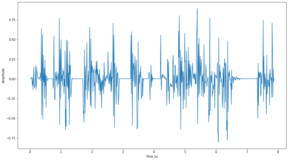
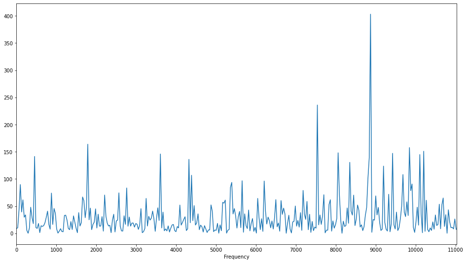
It's hard to figure out what's what just from these images but if we take a look at the Fourier transform of shorter second-long clips we start to get an idea about what frequencies correspond to what sounds in the audio clip.
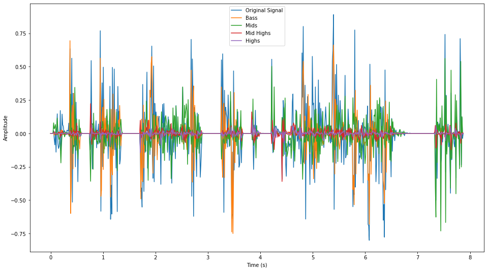
I implemented a bandpass filter to separate out all the frequencies so that they can be used separately to individually control different aspects of the morph sequence.
Now that we have the dials, we need to figure out what we want to tweak. Just to keep things simple for now, I decided to work with a smoothened signal (signal convolved with a 1D Gaussian filter) instead of working with all the components at the same time. I wanted to use the signal to control what frame of the A->B morph we're on. This is why it was important to smoothen the signal as without it consecutive frames of the morph could be quite different from each other due to high frequencies which would lead to jerky transitions. This is what the morph looked like using the smooth waveform synced to Boney M's Daddy Cool*
* i said bet, had to do it; warned you it might get weird
This doesn't look great. This was expected because it's only really keeping track of the soundwave amplitudes while ignoring the individual elements we actually percieve while listening to the music. I started thinking about all the ways I could improve on this, distort the faces through the frames into caricatures using the bass, have the high frequencies change the image hue while mids control the flow of the morph and trebble controls the rotation. All this sounds good but doesn't work. I implement a part of this and realized that it looked quite forced and wasn't as seemless as I was hoping/expecting it would be. Just because I had all these knobs for a face morph doesn't mean using them would make the result more pleasing. It was time to pivot.
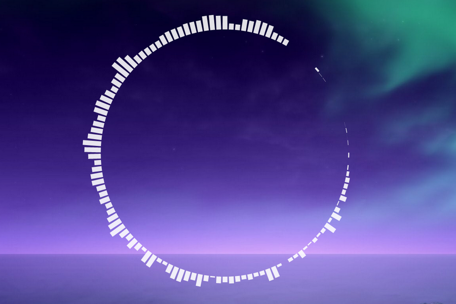
I quickly realized I had been constraining the idea by sticking to the face morphs when I could do so much more with the audio signal. I set out to implement a music visualizer, kinda like the ones that pop up in some Youtube videos. We want our final results to look something like this.
Now, we'll be working with all the frequencies of the signal instead of just the ones filtered out by our bandpass filters. We want to visualize how the frequencies of the audio clip change over time (spectrogram-like visualization). The visualization needs to show all the frequencies at each time step & smoothly transition between the frames. On top of that, I wanted the visualization to pulsate with the bass. First, we need to isolate the bass using a binary signal which encodes the locations of the bass. Implementing this bass detector took a lot of trial and error, but I finally got something that works. I looked at the fourier transforms of second-long clips and found out that the loud thumps in the clip belong to the frequency range ~10-60Hz. I used my bandpass filter to attentuate all other frequencies and then applied a threshold to the absolute value of the filtered signal. This gave me decent results but it still looked choppy so I convolved this with a box filter and then clipped the results to get nice smooth beat detections (shown below).
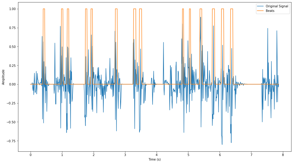
If you actually compare the postive regions to the audio clip above, you'll see this does a great job of picking the really loud thumps while ignoring other loud frequencies (Ex. 7-8s).
I found images for the base art and annotated them using automatically computed points along a circle. Each point along the circumference of the circle corresponds to a frequency and we scale the point according to the frequency's intensity at a given time step. Integrate this code with our image morphing code, throw in the beat detector and we have all the components for our visualizer. Time to see some results!
This took a hot second to implement & run so I think I'm going to stop here. There's still a lot that can be played around with. Things from changing color / transforming image shape based on certain frequency ranges to tracking the frequencies on a log scale to make the visualization more interpretable. I'll leave that to others to explore!
Final Takeaway
This project was genuinely super fun! I went in thinking that I'll just learn a bit about affine transformations but in an unexpected turn of events I ended up learning more singal processing than I did in EE16A & EE16B (time to take EE120 now??). The end results were ~perfectly splendid~ so I am quite happy :)